Gráficos Sankey con R

Gráficos Sankey con R

Hace unos días ví un informe con un tipo de gráficos poco habitual. Se trataba de una gráfica de flujo que se suelen denominar como diagramas de Sankey.

Se ha quedado con ese nombre por el ingeniero militar irlandés Matthew Henry Phineas Riall Sankey, que aunque no fue el inventor del gráfico, lo usó con acierto para una representación gráfica del flujo de energía en la máquina de vapor.

El caso es que me puse a buscar como hacer este tipo de gráficos en R y encontré una librería llamada networkD3 que, de manera sencilla, permite representar estos diagramas.

Como usar networkD3 para hacer un diagrama Sankey

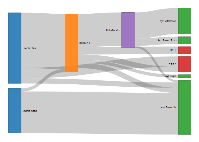
Lo mejor es que hagamos un ejemplo. Queremos representar el flujo de agua desde las fuentes a los abastecimientos y riegos en una zona y lo haremos con el diagrama Sankey y el paquete networkD3

Básicamente se trata de preparar los datos en una tabla de 3 columnas: origen, destino y volumen de flujo. También tendremos una tabla con los nombres de los nodos.

El código es el siguiente:

 # Ejemplo de diagrama de flujo SANKEY
 library(networkD3)      # cargamos librería
## Warning: package 'networkD3' was built under R version 4.0.5
 # Definimos los nodos de la red, que se numeran automáticamente de 0 a ..
 nodes = data.frame("name" = 
                   c("Fuente clara",  # Node 0
                     "Bombeo 1",      # Node 1
                     "Ayt. Villalocos",  # Node 2
                     "Ayt. Torrecilla",         # Nodo 3
                     "C.RR 1",        # Nodo 4
                     "C.RR 2",        # Nodo 5
                     "Embalse alto",  # Nodo 6
                     "Ayt. Puerto Plata", # Nodo 7
                     "Ayt. Jerjes",   # Nodo 8
                     "Fuente Negra"   # Nodo 9
                   ))
 # Definimos ahora los flujos en la forma siguiente:
 # nodo origen, nodo final, cantidad de flujo
 links = as.data.frame(matrix(c(
                        0, 1, 53, # desde, a, cuanto
                        0, 3, 5, 
                        0, 4, 10,
                        1, 3, 5,
                        1, 8, 3,
                        1, 5, 7,
                        1, 4, 5,
                        1, 6, 32,
                        6,2,25,
                        6,7,7,
                        6,3,2,
                        9,3,40,
                        9,1,3),
 byrow = TRUE, ncol = 3))
 # nombramos las columnas con los nombres estándar de la librería networkD3
  names(links) = c("source", "target", "value")
  # Llamamos a la funcion de dibujo del diagrama
  sankeyNetwork(Links = links, Nodes = nodes,
          Source = "source", Target = "target",
          Value = "value", NodeID = "name",
          fontSize= 10, nodeWidth = 50,nodePadding = 10,
          colourScale = JS("d3.scaleOrdinal(d3.schemeCategory10);"
          )
  )  
Fuente clara → Bombeo 1
53 
Fuente Negra → Ayt. Torrecilla
40 
Bombeo 1 → Embalse alto
32 
Embalse alto → Ayt. Villalocos
25 
Fuente clara → C.RR 1
10 
Bombeo 1 → C.RR 2
7 
Embalse alto → Ayt. Puerto Plata
7 
Fuente clara → Ayt. Torrecilla
5 
Bombeo 1 → Ayt. Torrecilla
5 
Bombeo 1 → C.RR 1
5 
Bombeo 1 → Ayt. Jerjes
3 
Fuente Negra → Bombeo 1
3 
Embalse alto → Ayt. Torrecilla
2 
Fuente clara
68
Fuente clara
Bombeo 1
56
Bombeo 1
Ayt. Villalocos
25
Ayt. Villalocos
Ayt. Torrecilla
52
Ayt. Torrecilla
C.RR 1
15
C.RR 1
C.RR 2
7
C.RR 2
Embalse alto
34
Embalse alto
Ayt. Puerto Plata
7
Ayt. Puerto Plata
Ayt. Jerjes
3
Ayt. Jerjes
Fuente Negra
43
Fuente Negra

Colorear flujo

Entre las opciones de la librería está el colorear los flujos, que se denominan Links.

Vamos a ver un ejemplo del gasto energético entre las fuentes de energía y los sectores que la gastan. Los datos originales son una tabla con: origen, destino, nombre, valor, del flujo, y tipo de energía.

  # Descargamos los datos 
    URL <- paste0('https://cdn.rawgit.com/christophergandrud/networkD3/',
          'master/JSONdata/energy.json')
    energy <- jsonlite::fromJSON(URL)
 
    #knitr::kable(head(energy),"html")
    str(energy)
## List of 2
##  $ nodes:'data.frame':   48 obs. of  1 variable:
##   ..$ name: chr [1:48] "Agricultural 'waste'" "Bio-conversion" "Liquid" "Losses" ...
##  $ links:'data.frame':   68 obs. of  3 variables:
##   ..$ source: int [1:68] 0 1 1 1 1 6 7 8 10 9 ...
##   ..$ target: int [1:68] 1 2 3 4 5 2 4 9 9 4 ...
##   ..$ value : num [1:68] 124.729 0.597 26.862 280.322 81.144 ...
    # Pintamos la grafica simple sin colorear flujos
    sankeyNetwork(Links = energy$links, Nodes = energy$nodes, Source = 'source',
          Target = 'target', Value = 'value', NodeID = 'name',
          units = 'TWh', fontSize = 12, nodeWidth = 30)
Nuclear → Thermal generation
840 TWh
Thermal generation → Losses
787 TWh
Oil → Liquid
612 TWh
Thermal generation → Electricity grid
526 TWh
Oil imports → Oil
504 TWh
Solid → Thermal generation
400 TWh
Electricity grid → Industry
342 TWh
Wind → Electricity grid
289 TWh
Bio-conversion → Solid
280 TWh
Liquid → International aviation
206 TWh
Pumped heat → Heating and cooling - homes
193 TWh
UK land based bioenergy → Bio-conversion
182 TWh
Gas → Thermal generation
152 TWh
Liquid → Road transport
136 TWh
Liquid → International shipping
129 TWh
Agricultural 'waste' → Bio-conversion
125 TWh
Ngas → Gas
123 TWh
Liquid → Industry
121 TWh
Electricity grid → Heating and cooling - homes
114 TWh
Oil reserves → Oil
108 TWh
Electricity grid → Over generation / exports
104 TWh
Electricity grid → Lighting & appliances - homes
93 TWh
Electricity grid → Lighting & appliances - commercial
90 TWh
Gas reserves → Ngas
82 TWh
Bio-conversion → Gas
81 TWh
Thermal generation → District heating
79 TWh
Other waste → Bio-conversion
78 TWh
Coal → Solid
76 TWh
Pumped heat → Heating and cooling - commercial
71 TWh
Coal reserves → Coal
64 TWh
Solar PV → Electricity grid
60 TWh
Solar → Solar PV
60 TWh
Electricity grid → Losses
57 TWh
Other waste → Solid
57 TWh
Gas → Industry
49 TWh
Solid → Industry
46 TWh
District heating → Heating and cooling - homes
46 TWh
Electricity grid → Heating and cooling - commercial
41 TWh
Gas imports → Ngas
41 TWh
Electricity grid → Road transport
38 TWh
Biofuel imports → Liquid
35 TWh
Biomass imports → Solid
35 TWh
Liquid → National navigation
33 TWh
Electricity grid → H2 conversion
27 TWh
Bio-conversion → Losses
27 TWh
District heating → Heating and cooling - commercial
23 TWh
H2 conversion → H2
21 TWh
H2 → Road transport
21 TWh
Solar Thermal → Heating and cooling - homes
19 TWh
Solar → Solar Thermal
19 TWh
Wave → Electricity grid
19 TWh
Liquid → Domestic aviation
14 TWh
Coal imports → Coal
12 TWh
District heating → Industry
11 TWh
Tidal → Electricity grid
9 TWh
Electricity grid → Rail transport
8 TWh
Geothermal → Electricity grid
7 TWh
Hydro → Electricity grid
7 TWh
H2 conversion → Losses
6 TWh
Liquid → Rail transport
4 TWh
Electricity grid → Agriculture
4 TWh
Marine algae → Bio-conversion
4 TWh
Liquid → Agriculture
4 TWh
Gas → Agriculture
2 TWh
Gas → Losses
1 TWh
Solid → Agriculture
1 TWh
Bio-conversion → Liquid
1 TWh
Gas → Heating and cooling - commercial
0 TWh
Agricultural 'waste'
125 TWh
Agricultural 'waste'
Bio-conversion
389 TWh
Bio-conversion
Liquid
648 TWh
Liquid
Losses
878 TWh
Losses
Solid
447 TWh
Solid
Gas
204 TWh
Gas
Biofuel imports
35 TWh
Biofuel imports
Biomass imports
35 TWh
Biomass imports
Coal imports
12 TWh
Coal imports
Coal
76 TWh
Coal
Coal reserves
64 TWh
Coal reserves
District heating
79 TWh
District heating
Industry
569 TWh
Industry
Heating and cooling - commercial
134 TWh
Heating and cooling - commercial
Heating and cooling - homes
372 TWh
Heating and cooling - homes
Electricity grid
919 TWh
Electricity grid
Over generation / exports
104 TWh
Over generation / exports
H2 conversion
27 TWh
H2 conversion
Road transport
195 TWh
Road transport
Agriculture
11 TWh
Agriculture
Rail transport
12 TWh
Rail transport
Lighting & appliances - commercial
90 TWh
Lighting & appliances - commercial
Lighting & appliances - homes
93 TWh
Lighting & appliances - homes
Gas imports
41 TWh
Gas imports
Ngas
123 TWh
Ngas
Gas reserves
82 TWh
Gas reserves
Thermal generation
1,392 TWh
Thermal generation
Geothermal
7 TWh
Geothermal
H2
21 TWh
H2
Hydro
7 TWh
Hydro
International shipping
129 TWh
International shipping
Domestic aviation
14 TWh
Domestic aviation
International aviation
206 TWh
International aviation
National navigation
33 TWh
National navigation
Marine algae
4 TWh
Marine algae
Nuclear
840 TWh
Nuclear
Oil imports
504 TWh
Oil imports
Oil
612 TWh
Oil
Oil reserves
108 TWh
Oil reserves
Other waste
134 TWh
Other waste
Pumped heat
264 TWh
Pumped heat
Solar PV
60 TWh
Solar PV
Solar Thermal
19 TWh
Solar Thermal
Solar
79 TWh
Solar
Tidal
9 TWh
Tidal
UK land based bioenergy
182 TWh
UK land based bioenergy
Wave
19 TWh
Wave
Wind
289 TWh
Wind
  # flujo coloreados
    energy$links$energy_type <- sub(' .*', '',
                            energy$nodes[energy$links$source + 1, 'name'])
  
    # los colores del flujo los definimos segun los valores de energy$links$energy_type
    knitr::kable(head(energy$links$energy_type))
x
Agricultural
Bio-conversion
Bio-conversion
Bio-conversion
Bio-conversion
Biofuel
  # pintamos la grafica con flujo coloreados
    sankeyNetwork(Links = energy$links, Nodes = energy$nodes, Source = 'source',
          Target = 'target', Value = 'value', NodeID = 'name',
          LinkGroup = 'energy_type', NodeGroup = NULL)
Nuclear → Thermal generation
840 
Thermal generation → Losses
787 
Oil → Liquid
612 
Thermal generation → Electricity grid
526 
Oil imports → Oil
504 
Solid → Thermal generation
400 
Electricity grid → Industry
342 
Wind → Electricity grid
289 
Bio-conversion → Solid
280 
Liquid → International aviation
206 
Pumped heat → Heating and cooling - homes
193 
UK land based bioenergy → Bio-conversion
182 
Gas → Thermal generation
152 
Liquid → Road transport
136 
Liquid → International shipping
129 
Agricultural 'waste' → Bio-conversion
125 
Ngas → Gas
123 
Liquid → Industry
121 
Electricity grid → Heating and cooling - homes
114 
Oil reserves → Oil
108 
Electricity grid → Over generation / exports
104 
Electricity grid → Lighting & appliances - homes
93 
Electricity grid → Lighting & appliances - commercial
90 
Gas reserves → Ngas
82 
Bio-conversion → Gas
81 
Thermal generation → District heating
79 
Other waste → Bio-conversion
78 
Coal → Solid
76 
Pumped heat → Heating and cooling - commercial
71 
Coal reserves → Coal
64 
Solar PV → Electricity grid
60 
Solar → Solar PV
60 
Electricity grid → Losses
57 
Other waste → Solid
57 
Gas → Industry
49 
Solid → Industry
46 
District heating → Heating and cooling - homes
46 
Electricity grid → Heating and cooling - commercial
41 
Gas imports → Ngas
41 
Electricity grid → Road transport
38 
Biofuel imports → Liquid
35 
Biomass imports → Solid
35 
Liquid → National navigation
33 
Electricity grid → H2 conversion
27 
Bio-conversion → Losses
27 
District heating → Heating and cooling - commercial
23 
H2 conversion → H2
21 
H2 → Road transport
21 
Solar Thermal → Heating and cooling - homes
19 
Solar → Solar Thermal
19 
Wave → Electricity grid
19 
Liquid → Domestic aviation
14 
Coal imports → Coal
12 
District heating → Industry
11 
Tidal → Electricity grid
9 
Electricity grid → Rail transport
8 
Geothermal → Electricity grid
7 
Hydro → Electricity grid
7 
H2 conversion → Losses
6 
Liquid → Rail transport
4 
Electricity grid → Agriculture
4 
Marine algae → Bio-conversion
4 
Liquid → Agriculture
4 
Gas → Agriculture
2 
Gas → Losses
1 
Solid → Agriculture
1 
Bio-conversion → Liquid
1 
Gas → Heating and cooling - commercial
0 
Agricultural 'waste'
125
Agricultural 'waste'
Bio-conversion
389
Bio-conversion
Liquid
648
Liquid
Losses
878
Losses
Solid
447
Solid
Gas
204
Gas
Biofuel imports
35
Biofuel imports
Biomass imports
35
Biomass imports
Coal imports
12
Coal imports
Coal
76
Coal
Coal reserves
64
Coal reserves
District heating
79
District heating
Industry
569
Industry
Heating and cooling - commercial
134
Heating and cooling - commercial
Heating and cooling - homes
372
Heating and cooling - homes
Electricity grid
919
Electricity grid
Over generation / exports
104
Over generation / exports
H2 conversion
27
H2 conversion
Road transport
195
Road transport
Agriculture
11
Agriculture
Rail transport
12
Rail transport
Lighting & appliances - commercial
90
Lighting & appliances - commercial
Lighting & appliances - homes
93
Lighting & appliances - homes
Gas imports
41
Gas imports
Ngas
123
Ngas
Gas reserves
82
Gas reserves
Thermal generation
1,392
Thermal generation
Geothermal
7
Geothermal
H2
21
H2
Hydro
7
Hydro
International shipping
129
International shipping
Domestic aviation
14
Domestic aviation
International aviation
206
International aviation
National navigation
33
National navigation
Marine algae
4
Marine algae
Nuclear
840
Nuclear
Oil imports
504
Oil imports
Oil
612
Oil
Oil reserves
108
Oil reserves
Other waste
134
Other waste
Pumped heat
264
Pumped heat
Solar PV
60
Solar PV
Solar Thermal
19
Solar Thermal
Solar
79
Solar
Tidal
9
Tidal
UK land based bioenergy
182
UK land based bioenergy
Wave
19
Wave
Wind
289
Wind

Esto es todo amigos.